Fringe Examples

by Peter John Smith

You should read up on types of Interferometers and their use.

(Note that Fringe-XP cannot analyze Interferograms from a 'Shearing Interferometer' but will handle those from most others and the Fizeau type as popularized by Peter Ceravolo for ATM use.)
The following 'interferograms' have been taken with a typical red laser source with a wavelength of 633 nm.l

A Hindle Sphere

Let's investigate the accuracy of a Simulated Hindle Sphere using Fringe-XP This Synthetic Interferogram is called 'sphere_hindle.jpg' Load the following jpg picture into Fringe-XP, either from the original file, or by copying from the picture below in this document.

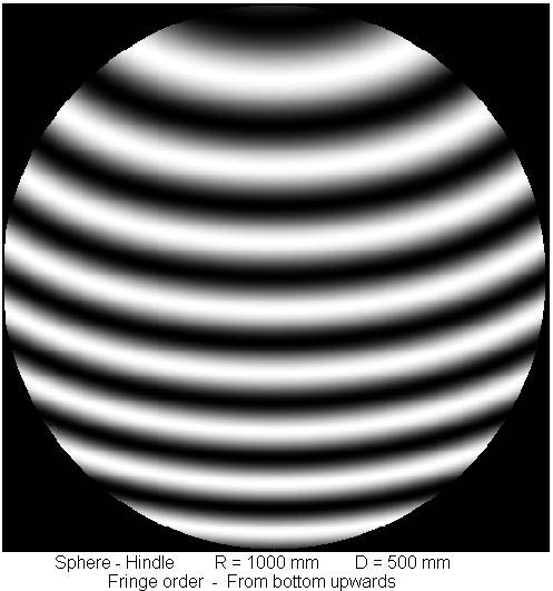
The Fringe order is from the bottom up.

Thus, if you enter the points for the bottom fringe first and increment to the next higher fringe, the fringe spacing to be entered into Fringe-XP is either + 0.5 or + 1.0, depending on whether you enter both the light and dark fringes, or simply alternate fringes of the same colour.

You should derive Zernike Coefficients very similar to those below.

They will not be identical, because the entered points are not exactly the same.

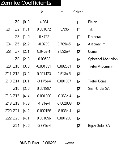
Close examination of these values gives clues about the surface, and how we should approach a surface analysis.

Most of these terms are close to zero.

The first term, Z0, is 'Piston' which can be ignored. It is not a property of the surface.

The next two terms may also be ignored. The Y tilt is close to 4. This is related to the number of fringes across the surface which may be changed by adjusting the 'tilt' when we set up the interferometer. This is not a property of the surface, so is deselected from the surface analysis.

The fourth term - Z4 - also depends on the setup of the Interferometer so may be ignored except in one case.

Defocus introduces more curvature to the fringes and may result in a large bulls-eye pattern. It is best removed as much as possible during the setup of the interferometer. In this case, if the interferometer had been perfectly adjusted, near straight fringes would have resulted. Defocus does not matter, within reason, because we can extract this setup defect during analysis.

The only exception is when flats are tested when any defocus term must be included.

This is not the case here, so we will have it deselected in the surface analysis.

Examination of the other terms shows that the only other significant coefficients are :-

Z4 - an Astigmatism term.

Z8 - a small amount of primary Spherical Aberration.

The first to ponder is the Z4 = -.078 Astigmatism term. It is very evident from the Contour Plot, that the surface is 'folded' somewhat which accounts for most of the error.

Remember to set the Target Conic = 0, R = 1000, D = 500 mm. and the Reporting wavelength to something sensible such as 550 nm for Visual use when doing the Surface Analysis.

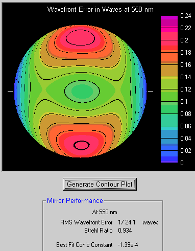
Your Contour plot will be slightly different. The total wavefront deviation is about 0.2 waves so the surface deviation is about 0.1 wave.

If this is caused by bending of the mirror relating to mounting it, then a better mounting system may produce a very useable Hindle Sphere. If the Astigmatism is polished into the glass it's a fairly good Sphere, but maybe not good enough for testing Cassegrainian secondaries.

Fortunately, by rotating the mirror on its mounts to different positions, and taking many Interferograms, we can deduce whether the fault is in the surface or mounting.

If the surface really has no Astigmatism, how good is it?

Deselect the Astigmatism terms and do an analysis.

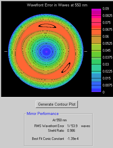
The Contour plot looks colourful and wild. But, on closer examination, the scale is such that the surface is excellent.

It's definitely a very good Hindle Sphere - as long as the Astigmatism can be eliminated by more careful mirror support.

A Parabola?

See if you concur with the summaries of the Interferogram below.

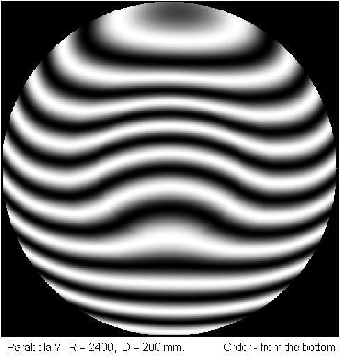
This is labeled Parabola-Maybe.jpg

Examination of the Zernike Coefficients reveals the following terms may be worth investigating.

Z4, Z5, Z10 (Astigmatism)

Z6, Z7 (Coma)

Z8, Z15, Z24 (Spherical Aberration)

Do not forget to set the values of Wavelengths, R, D and the Target Conic of -1.0 as appropriate for a Parabola.

The following plots show a symmetric deformation about the 150 degree axis, and a non symmetric deformation along this axis.

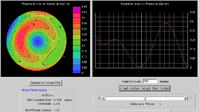
It is almost certain that Coma has been introduced by a slightly off axis setting when the Interferogram was taken. When the mirror is used in a telescope, the 'Coma' should be eliminated by appropriate alignment adjustments.

If so, it is quite valid to deselect the Coma terms and re-evaluate the surface.

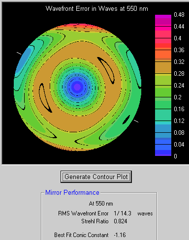
We now see an overcorrected Parabola, with a small amount of Astigmatism.

It would perform reasonably in a Telescope, but many would wish for something better.

If the Astigmatism is caused by mounting problems, we can also deselect Z4, Z5 and possibly some other terms. This raises the Strehl Ratio to 0.85. Although the PV wavefront range is about 0.4 (on the surface 0.2), the Strehl value is a far better indicator of performance.

What about the Z8, Z15, Z24 terms (Spherical Aberration)?

Since it is a 'Parabola' tested at Centre of Curvature, the wavefront seen by the Interferometer should contain Spherical Aberration. By specifying a Conic Target of -1, Fringe-XP is in effect comparing this with the Spherical Aberration which should be present.

Many would attempt to improve this surface. You may wish to investigate future figuring strategies using the Defocus adjustment.